1 Introduction

Functional verification constitutes one of the most challenging and time-consuming steps in the design of modern digital systems. The primary objective of functional verification is to expose design bugs early in the design cycle. Among various techniques available for this purpose, those based on simulation overwhelmingly dominate industrial practice. In a typical simulation-based functional verification exercise, a gate-level or RTL model of the circuit is simulated for a large number of cycles with specific input patterns. The values at observable outputs, as computed by the simulator, are then compared against their expected values, and any discrepancy is flagged as manifestaton of a bug. The state of simulation technology today is mature enough to allow simulation of large designs within reasonable time using modest computational resources. Generating input patterns that exercise diverse corners of the design’s behavior space, however, remains a challenging problem [4].

In recent years, constrained-random simulation (also called constrained-random verification, or CRV) [21] has emerged as a practical approach to address the problem of simulating designs with “random enough” input patterns. In CRV, the verification engineer declaratively specifies a set of constraints on the values of circuit inputs. Typically, these constraints are obtained from usage requirements, environmental constraints, constraints on operating conditions and the like. A constraint solver is then used to generate random values for the circuit inputs satisfying the constraints. Since the distribution of errors in the design’s behavior space is not known a priori, every solution to the set of constraints is as likely to discover a bug as any other solution. It is therefore important to sample the space of all solutions uniformly or almost-uniformly (defined formally below) at random. Unfortunately, guaranteeing uniformity poses significant technical challenges when scaling to large problem sizes. This has been repeatedly noted in the literature (see, for example, [8, 22, 16]) and also confirmed by industry practitioners. The difficulties of generating solutions with guarantees of uniformity have even prompted researchers to propose alternative techniques for generating input patterns [8, 22]. This paper takes a step towards remedying this situation. Specifically, we describe an algorithm for generating solutions to a set of Boolean constraints, with stronger guarantees on uniformity and with higher scalability in practice than that achieved earlier.

Since constraints that arise in CRV of digital circuits are encodable as Boolean formulae, we focus on uniform generation of solutions of Boolean formulae. Henceforth, we call such solutions 𝖲𝖠𝖳𝖲𝖠𝖳\mathsf{SAT} witnesses. Besides its usefulness in CRV and in other applications [2, 23], uniform generation of SAT witnesses has had strong theoretical interest as well [14]. Most prior approaches to solving this problem belong to one of two categories: those that focus on strong guarantees of uniformity but scale poorly in practice (examples being [27, 3, 14]), and those that provide practical heuristics to scale to large problem instances with weak or no guarantees of uniformity (examples being [7, 16, 25])). In [5], Chakraborty, Meel and Vardi attempted to bridge these extremes through an algorithm called 𝖴𝗇𝗂𝖶𝗂𝗍𝖴𝗇𝗂𝖶𝗂𝗍\mathsf{UniWit}. More recently, Ermon, Gomes, Sabharwal and Selman [9] proposed an algorithm called 𝖯𝖠𝖶𝖲𝖯𝖠𝖶𝖲\mathsf{PAWS} for sampling witnesses from discrete distributions over large dimensions. While 𝖯𝖠𝖶𝖲𝖯𝖠𝖶𝖲\mathsf{PAWS} is designed to work with any discrete distribution specified through a graphical model, for purposes of this paper, we focus only on distributions that assign equal weight to every assignment. For such distributions, both 𝖯𝖠𝖶𝖲𝖯𝖠𝖶𝖲\mathsf{PAWS} and 𝖴𝗇𝗂𝖶𝗂𝗍𝖴𝗇𝗂𝖶𝗂𝗍\mathsf{UniWit} represent alternative (albeit related) approaches to solve the same problem – that of uniform generation of SAT witnesses. Unfortunately, both algorithms suffer from inherent limitations that make it difficult to scale them to Boolean constraints with tens of thousands of variables and beyond. In addition, the guarantees provided by these algorithms (in the context of uniform generation of SAT witnesses) are weaker than what one would desire in practice.

In this paper, we propose an algorithm called 𝖴𝗇𝗂𝖦𝖾𝗇𝖴𝗇𝗂𝖦𝖾𝗇\mathsf{UniGen} that addresses some of the deficiencies of 𝖴𝗇𝗂𝖶𝗂𝗍𝖴𝗇𝗂𝖶𝗂𝗍\mathsf{UniWit} and 𝖯𝖠𝖶𝖲𝖯𝖠𝖶𝖲\mathsf{PAWS}. This enables us to improve both the theoretical guarantees and practical performance vis-a-vis earlier algorithms in the context of uniform generation of SAT witnesses. 𝖴𝗇𝗂𝖦𝖾𝗇𝖴𝗇𝗂𝖦𝖾𝗇\mathsf{UniGen} is the first algorithm to provide strong two-sided guarantees of almost-uniformity, while scaling to problems involving hundreds of thousands of variables. We also improve upon the success probability of the earlier algorithms significantly, both in theory and as evidenced by our experiments.

2 Notation and Preliminaries

Let F𝐹F be a Boolean formula in conjunctive normal form (CNF), and let X𝑋X be the set of variables appearing in F𝐹F. The set X𝑋X is called the support of F𝐹F. A satisfying assignment or witness of F𝐹F is an assignment of truth values to variables in its support such that F𝐹F evaluates to true. We denote the set of all witnesses of F𝐹F as RFsubscript𝑅𝐹R_{F}. Let 𝒟⊆X𝒟𝑋{\mathcal{D}}\subseteq X be a subset of the support such that there are no two satisfying assignments of F𝐹F that differ only in the truth values of variables in 𝒟𝒟{\mathcal{D}}. In other words, in every satisfying assignment of F𝐹F, the truth values of variables in X∖𝒟𝑋𝒟X\setminus{\mathcal{D}} uniquely determine the truth value of every variable in 𝒟𝒟{\mathcal{D}}. The set 𝒟𝒟{\mathcal{D}} is called a dependent support of F𝐹F, and X∖𝒟𝑋𝒟X\setminus\mathcal{D} is called an independent support of F𝐹F. Note that there may be more than one independent supports of F𝐹F. For example, (a∨¬b)∧(¬a∨b)𝑎𝑏𝑎𝑏(a\vee\neg b)\wedge(\neg a\vee b) has three independent supports: {a}𝑎{a}, {b}𝑏{b} and {a,b}𝑎𝑏{a,b}. Clearly, if ℐℐ{\mathcal{I}} is an independent support of F𝐹F, so is every superset of ℐℐ{\mathcal{I}}. For notational convenience, whenever the formula F𝐹F is clear from the context, we omit mentioning it.

We use 𝖯𝗋[X:𝒫]\mathsf{Pr}\left[X:{\cal P}\right] to denote the probability of outcome X𝑋X when sampling from a probability space 𝒫𝒫{\cal P}. For notational clarity, we omit 𝒫𝒫{\cal P} when it is clear from the context. The expected value of the outcome X𝑋X is denoted 𝖤​[X]𝖤delimited-[]𝑋\mathsf{E}\left[X\right]. Given a Boolean formula F𝐹F, a probabilistic generator of witnesses of F𝐹F is a probabilistic algorithm that generates a random witness in RFsubscript𝑅𝐹R_{F}. A uniform generator 𝒢u​(⋅)superscript𝒢𝑢⋅\mathcal{G}^{u}(\cdot) is a probabilistic generator that guarantees 𝖯𝗋​[𝒢u​(F)=y]=1/|RF|𝖯𝗋delimited-[]superscript𝒢𝑢𝐹𝑦1subscript𝑅𝐹\mathsf{Pr}\left[\mathcal{G}^{u}(F)=y\right]=1/|R_{F}|, for every y∈RF𝑦subscript𝑅𝐹y\in R_{F}. An almost-uniform generator 𝒢a​u​(⋅,⋅)superscript𝒢𝑎𝑢⋅⋅\mathcal{G}^{au}(\cdot,\cdot) ensures that for every y∈RF𝑦subscript𝑅𝐹y\in R_{F}, we have 1(1+ε)​|RF|11𝜀subscript𝑅𝐹\frac{1}{(1+\varepsilon)|R_{F}|} ≤\leq 𝖯𝗋​[𝒢a​u​(F,ε)=y]≤𝖯𝗋delimited-[]superscript𝒢𝑎𝑢𝐹𝜀𝑦absent\mathsf{Pr}\left[\mathcal{G}^{au}(F,\varepsilon)=y\right]\leq 1+ε|RF|1𝜀subscript𝑅𝐹\frac{1+\varepsilon}{|R_{F}|}, where ε>0𝜀0\varepsilon>0 is the specified tolerance. A near-uniform generator 𝒢n​u​(⋅)superscript𝒢𝑛𝑢⋅\mathcal{G}^{nu}(\cdot) further relaxes the guarantee of uniformity, and ensures that 𝖯𝗋​[𝒢n​u​(F)=y]≥c/|RF|𝖯𝗋delimited-[]superscript𝒢𝑛𝑢𝐹𝑦𝑐subscript𝑅𝐹\mathsf{Pr}\left[\mathcal{G}^{nu}(F)=y\right]\geq c/|R_{F}| for a constant c𝑐c, where 0<c≤10𝑐10<c\leq 1. Probabilistic generators are allowed to occasionally “fail" in the sense that no witness may be returned even if RFsubscript𝑅𝐹R_{F} is non-empty. The failure probability for such generators must be bounded by a constant strictly less than 1. The algorithm presented in this paper falls in the category of almost-uniform generators. An idea closely related to that of almost-uniform generation, and used in a key manner in our algorithm, is *approximate model counting*. Given a CNF formula F𝐹F, an *exact model counter* returns the size of RFsubscript𝑅𝐹R_{F}. An *approximate model counter* 𝖠𝗉𝗉𝗋𝗈𝗑𝖬𝖢​(⋅,⋅,⋅)𝖠𝗉𝗉𝗋𝗈𝗑𝖬𝖢⋅⋅⋅{\mathsf{ApproxMC}}(\cdot,\cdot,\cdot) relaxes this requirement to some extent. Given a CNF formula F𝐹F, a tolerance ε>0𝜀0\varepsilon>0 and a confidence 1−δ∈(0,1]1𝛿011-\delta\in(0,1], and approximate model counter ensures that 𝖯𝗋​[|RF|1+ε≤𝖠𝗉𝗉𝗋𝗈𝗑𝖬𝖢​(F,ε,1−δ)≤(1+ε)​|RF|]≥1−δ𝖯𝗋delimited-[]subscript𝑅𝐹1𝜀𝖠𝗉𝗉𝗋𝗈𝗑𝖬𝖢𝐹𝜀1𝛿1𝜀subscript𝑅𝐹1𝛿\mathsf{Pr}[\frac{|R_{F}|}{1+\varepsilon}\leq{\mathsf{ApproxMC}}(F,\varepsilon,1-\delta)\leq(1+\varepsilon)|R_{F}|]\geq 1-\delta.

A special class of hash functions, called r𝑟r-wise independent hash functions, play a crucial role in our work. Let n,m

𝑛𝑚n,m and r𝑟r be positive integers, and let H​(n,m,r)𝐻𝑛𝑚𝑟H(n,m,r) denote a family of r𝑟r-wise independent hash functions mapping {0,1}nsuperscript01𝑛{0,1}^{n} to {0,1}msuperscript01𝑚{0,1}^{m}. We use h←𝑅H​(n,m,r)𝑅←ℎ𝐻𝑛𝑚𝑟h\xleftarrow{R}H(n,m,r) to denote the probability space obtained by choosing a hash function hℎh uniformly at random from H​(n,m,r)𝐻𝑛𝑚𝑟H(n,m,r). The property of r𝑟r-wise independence guarantees that for all α1,…​αr∈{0,1}m

subscript𝛼1…subscript𝛼𝑟 superscript01𝑚\alpha_{1},\ldots\alpha_{r}\in{0,1}^{m} and for all distinct y1,…​yr∈{0,1}n

subscript𝑦1…subscript𝑦𝑟 superscript01𝑛y_{1},\ldots y_{r}\in{0,1}^{n}, 𝖯𝗋[⋀i=1rh(yi)=αi\mathsf{Pr}\left[\bigwedge_{i=1}^{r}h(y_{i})=\alpha_{i}\right. :h←𝑅H(n,m,r)]=2−m​r\left.:h\xleftarrow{R}H(n,m,r)\right]=2^{-mr}. For every α∈{0,1}m𝛼superscript01𝑚\alpha\in{0,1}^{m} and h∈H​(n,m,r)ℎ𝐻𝑛𝑚𝑟h\in H(n,m,r), let h−1​(α)superscriptℎ1𝛼h^{-1}(\alpha) denote the set {y∈{0,1}n∣h​(y)=α}conditional-set𝑦superscript01𝑛ℎ𝑦𝛼{y\in{0,1}^{n}\mid h(y)=\alpha}. Given RF⊆{0,1}nsubscript𝑅𝐹superscript01𝑛R_{F}\subseteq{0,1}^{n} and h∈H​(n,m,r)ℎ𝐻𝑛𝑚𝑟h\in H(n,m,r), we use RF,h,αsubscript𝑅

𝐹ℎ𝛼R_{F,h,\alpha} to denote the set RF∩h−1​(α)subscript𝑅𝐹superscriptℎ1𝛼R_{F}\cap h^{-1}(\alpha). If we keep hℎh fixed and let α𝛼\alpha range over {0,1}msuperscript01𝑚{0,1}^{m}, the sets RF,h,αsubscript𝑅

𝐹ℎ𝛼R_{F,h,\alpha} form a partition of RFsubscript𝑅𝐹R_{F}.

3 Related Work

Marrying scalability with strong guarantees of uniformity has been the holy grail of algorithms that sample from solutions of constraint systems. The literature bears testimony to the significant tension between these objectives when designing random generators of SAT witnesses. Earlier work in this area either provide strong theoretical guarantees at the cost of scalability, or remedy the scalability problem at the cost of guarantees of uniformity. More recently, however, there have been efforts to bridge these two extremes.

Bellare, Goldreich and Petrank [3] showed that a provably uniform generator of SAT witnesses can be designed in theory to run in probabilistic polynomial time relative to an 𝖭𝖯𝖭𝖯\mathsf{NP} oracle. Unfortunately, it was shown in [5] that this algorithm does not scale beyond formulae with few tens of variables in practice. Weighted binary decision diagrams (BDD) have been used in [27] to sample uniformly from SAT witnesses. However, BDD-based techniques are known to suffer from scalability problems [16]. Adapted BDD-based techniques with improved performance were proposed in [18]; however, the scalability was achieved at the cost of guarantees of uniformity. Random seeding of DPLL SAT solvers [20] has been shown to offer performance, although the generated distributions of witnesses can be highly skewed [16].

Markov Chain Monte Carlo methods (also called MCMC methods) [16, 26] are widely considered to be a practical way to sample from a distribution of solutions. Several MCMC algorithms, such as those based on simulated annealing, Metropolis-Hastings algorithm and the like, have been studied extensively in the literature [15, 19]. While MCMC methods guarantee eventual convergence to a target distribution under mild requirements, convergence is often impractically slow in practice. The work of [26, 16] proposed several such adaptations for MCMC-based sampling in the context of constrained-random verification. Unfortunately, most of these adaptations are heuristic in nature, and do not preserve theoretical guarantees of uniformity. constraints, thereby increasing constraint-solving time. Sampling techniques based on interval-propagation and belief networks have been proposed in [7, 10, 13]. The simplicity of these approaches lend scalability to the techniques, but the generated distributions can deviate significantly from the uniform distribution, as shown in [17].

Sampling techniques based on hashing were originally pioneered by Sipser [24], and have been used subsequently by several researchers [3, 11, 5]. The core idea in hashing-based sampling is to use r𝑟r-wise independent hash functions (for a suitable value of r𝑟r) to randomly partition the space of witnesses into “small cells" of roughly equal size, and then randomly pick a solution from a randomly chosen cell. The algorithm of Bellare et al. referred to above uses this idea with n𝑛n-wise independent algebraic hash functions (where n𝑛n denotes the size of the support of F𝐹F). As noted above, their algorithm scales very poorly in practice. Gomes, Sabharwal and Selman used 333-wise independent linear hash functions in [11] to design 𝖷𝖮𝖱𝖲𝖺𝗆𝗉𝗅𝖾′superscript𝖷𝖮𝖱𝖲𝖺𝗆𝗉𝗅𝖾′\mathsf{XORSample}^{\prime}, a near-uniform generator of SAT witnesses. Nevertheless, to realize the guarantee of near-uniformity, their algorithm requires the user to provide difficult-to-estimate input parameters. Although 𝖷𝖮𝖱𝖲𝖺𝗆𝗉𝗅𝖾′superscript𝖷𝖮𝖱𝖲𝖺𝗆𝗉𝗅𝖾′\mathsf{XORSample}^{\prime} has been shown to scale to constraints involving a few thousand variables, Gomes et al. acknowledge the difficulty of scaling their algorithm to much larger problem sizes without sacrificing theoretical guarantees [11].

Recently, Chakraborty, Meel and Vardi [5] proposed a new hashing-based SAT witness generator, called 𝖴𝗇𝗂𝖶𝗂𝗍𝖴𝗇𝗂𝖶𝗂𝗍\mathsf{UniWit}, that represents a small but significant step towards marrying the conflicting goals of scalability and guarantees of uniformity. Like 𝖷𝖮𝖱𝖲𝖺𝗆𝗉𝗅𝖾′superscript𝖷𝖮𝖱𝖲𝖺𝗆𝗉𝗅𝖾′\mathsf{XORSample}^{\prime}, the 𝖴𝗇𝗂𝖶𝗂𝗍𝖴𝗇𝗂𝖶𝗂𝗍\mathsf{UniWit} algorithm uses 333-wise independent linear hashing functions. Unlike 𝖷𝖮𝖱𝖲𝖺𝗆𝗉𝗅𝖾′superscript𝖷𝖮𝖱𝖲𝖺𝗆𝗉𝗅𝖾′\mathsf{XORSample}^{\prime}, however, the guarantee of near-uniformity of witnesses generated by 𝖴𝗇𝗂𝖶𝗂𝗍𝖴𝗇𝗂𝖶𝗂𝗍\mathsf{UniWit} does not depend on difficult-to-estimate input parameters. In [5], 𝖴𝗇𝗂𝖶𝗂𝗍𝖴𝗇𝗂𝖶𝗂𝗍\mathsf{UniWit} has been shown to scale to formulas with several thousand variables. In addition, Chakraborty et al proposed a heuristic called “leap-frogging” that allows 𝖴𝗇𝗂𝖶𝗂𝗍𝖴𝗇𝗂𝖶𝗂𝗍\mathsf{UniWit} to scale even further – to tens of thousands of variables [5]. Unfortunately, the guarantees of near-uniformity can no longer be established for 𝖴𝗇𝗂𝖶𝗂𝗍𝖴𝗇𝗂𝖶𝗂𝗍\mathsf{UniWit} with “leap-frogging”. More recently, Ermon et al. [9] proposed a hashing-based algorithm called 𝖯𝖠𝖶𝖲𝖯𝖠𝖶𝖲\mathsf{PAWS} for sampling from a distribution defined over a discrete set using a graphical model. While the algorithm presented in this paper has some similarities with 𝖯𝖠𝖶𝖲𝖯𝖠𝖶𝖲\mathsf{PAWS}, there are significant differences as well. Specifically, our algorithm provides much stronger theoretical guarantees vis-a-vis those offered by 𝖯𝖠𝖶𝖲𝖯𝖠𝖶𝖲\mathsf{PAWS} in the context of uniform generation of SAT witness. In addition, our algorithm scales to hundreds of thousands of variables while preserving the theoretical guarantees. 𝖯𝖠𝖶𝖲𝖯𝖠𝖶𝖲\mathsf{PAWS} faces the same scalability hurdles as 𝖴𝗇𝗂𝖶𝗂𝗍𝖴𝗇𝗂𝖶𝗂𝗍\mathsf{UniWit}, and is unlikely to scale beyond a few thousand variables without heuristic adapatations that compromise its guarantees.

4 The UniGen Algorithm

The new algorithm, called 𝖴𝗇𝗂𝖦𝖾𝗇𝖴𝗇𝗂𝖦𝖾𝗇\mathsf{UniGen}, falls in the category of hashing-based almost-uniform generators. 𝖴𝗇𝗂𝖦𝖾𝗇𝖴𝗇𝗂𝖦𝖾𝗇\mathsf{UniGen} shares some features with earlier hashing-based algorithms such as 𝖷𝖮𝖱𝖲𝖺𝗆𝗉𝗅𝖾′superscript𝖷𝖮𝖱𝖲𝖺𝗆𝗉𝗅𝖾′\mathsf{XORSample}^{\prime} [11], 𝖴𝗇𝗂𝖶𝗂𝗍𝖴𝗇𝗂𝖶𝗂𝗍\mathsf{UniWit} [5] and 𝖯𝖠𝖶𝖲𝖯𝖠𝖶𝖲\mathsf{PAWS} [9], but there are key differences that allow 𝖴𝗇𝗂𝖦𝖾𝗇𝖴𝗇𝗂𝖦𝖾𝗇\mathsf{UniGen} to significantly outperform these earlier algorithms, both in terms of theoretical guarantees and measured performance.

Given a CNF formula F𝐹F, we use a family of 333-independent hash functions to randomly partition the set, RFsubscript𝑅𝐹R_{F}, of witnesses of F𝐹F. Let h:{0,1}n→{0,1}m:ℎ→superscript01𝑛superscript01𝑚h:{0,1}^{n}\rightarrow{0,1}^{m} be a hash function in the family, and let y𝑦y be a vector in {0,1}nsuperscript01𝑛{0,1}^{n}. Let h​(y)​[i]ℎ𝑦delimited-[]𝑖h(y)[i] denote the it​hsuperscript𝑖𝑡ℎi^{th} component of the vector obtained by applying hℎh to y𝑦y. The family of hash functions of interest is defined as {h​(y)∣h​(y)​[i]=ai,0⊕(⨁k=1nai,k⋅y​[k]),ai,j∈{0,1},1≤i≤m,0≤j≤n}conditional-setℎ𝑦formulae-sequenceformulae-sequenceℎ𝑦delimited-[]𝑖direct-sumsubscript𝑎

𝑖0superscriptsubscriptdirect-sum𝑘1𝑛⋅subscript𝑎

𝑖𝑘𝑦delimited-[]𝑘formulae-sequencesubscript𝑎

𝑖𝑗011𝑖𝑚0𝑗𝑛{h(y)\mid h(y)[i]=a_{i,0}\oplus(\bigoplus_{k=1}^{n}a_{i,k}\cdot y[k]),a_{i,j}\in{0,1},1\leq i\leq m,0\leq j\leq n}, where ⊕direct-sum\oplus denotes the xor operation. By choosing values of ai,jsubscript𝑎

𝑖𝑗a_{i,j} randomly and independently, we can effectively choose a random hash function from the family. It has been shown in [11] that this family of hash functions is 333-independent. Following notation introduced in Section 2, we call this family Hx​o​r​(n,m,3)subscript𝐻𝑥𝑜𝑟𝑛𝑚3H_{xor}(n,m,3).

While Hx​o​r​(n,m,3)subscript𝐻𝑥𝑜𝑟𝑛𝑚3H_{xor}(n,m,3) was used earlier in 𝖷𝖮𝖱𝖲𝖺𝗆𝗉𝗅𝖾′superscript𝖷𝖮𝖱𝖲𝖺𝗆𝗉𝗅𝖾′\mathsf{XORSample}^{\prime}, 𝖯𝖠𝖶𝖲𝖯𝖠𝖶𝖲\mathsf{PAWS}, and (in a variant of) 𝖴𝗇𝗂𝖶𝗂𝗍𝖴𝗇𝗂𝖶𝗂𝗍\mathsf{UniWit}, there is a fundamental difference in the way we use it in 𝖴𝗇𝗂𝖦𝖾𝗇𝖴𝗇𝗂𝖦𝖾𝗇\mathsf{UniGen}. Let X={x1,x2,…​x|X|}𝑋subscript𝑥1subscript𝑥2…subscript𝑥𝑋X={x_{1},x_{2},\ldots x_{|X|}} be the set of variables of F𝐹F. Given m>0𝑚0m>0, the algorithms 𝖷𝖮𝖱𝖲𝖺𝗆𝗉𝗅𝖾′superscript𝖷𝖮𝖱𝖲𝖺𝗆𝗉𝗅𝖾′\mathsf{XORSample}^{\prime}, 𝖯𝖠𝖶𝖲𝖯𝖠𝖶𝖲\mathsf{PAWS} and 𝖴𝗇𝗂𝖶𝗂𝗍𝖴𝗇𝗂𝖶𝗂𝗍\mathsf{UniWit} partition RFsubscript𝑅𝐹R_{F} by randomly choosing h∈Hx​o​r​(|X|,m,3)ℎsubscript𝐻𝑥𝑜𝑟𝑋𝑚3h\in H_{xor}(|X|,m,3) and α∈{0,1}m𝛼superscript01𝑚\alpha\in{0,1}^{m}, and by seeking witnesses of F𝐹F conjoined with ⋀i=1m(h(x1,…x|X|)[i]↔α[i])\bigwedge_{i=1}^{m}\left(h(x_{1},\ldots x_{|X|})[i]\leftrightarrow\alpha[i]\right). By choosing a random h​(x1,…​x|X|)∈Hx​o​r​(|X|,m,3)ℎsubscript𝑥1…subscript𝑥𝑋subscript𝐻𝑥𝑜𝑟𝑋𝑚3h(x_{1},\ldots x_{|X|})\in H_{xor}(|X|,m,3), the set of all assignments to variables in X𝑋X (regardless of whether they are witnesses of F𝐹F) is partitioned randomly. This, in turn, ensures that the set of satisfying assignments of F𝐹F is also partitioned randomly. Each conjunctive constraint of the form (h(x1…x|X|)[i](https://ar5iv.labs.arxiv.org/html/h(x_{1}\ldots x_{|X|})[i] ↔↔\leftrightarrow α[i])\alpha[i]) is an xor of a subset of variables of X𝑋X and α​[i]𝛼delimited-[]𝑖\alpha[i], and is called an xor-clause. Observe that the expected number of variables in each such xor-clause is approximately |X|/2𝑋2|X|/2. It is well-known (see, for example [12]) that the difficulty of checking satisfiability of a CNF formula with xor-clauses grows significantly with the number of variables per xor-clause. It is therefore extremely difficult to scale 𝖷𝖮𝖱𝖲𝖺𝗆𝗉𝗅𝖾′superscript𝖷𝖮𝖱𝖲𝖺𝗆𝗉𝗅𝖾′\mathsf{XORSample}^{\prime}, 𝖯𝖠𝖶𝖲𝖯𝖠𝖶𝖲\mathsf{PAWS} or 𝖴𝗇𝗂𝖶𝗂𝗍𝖴𝗇𝗂𝖶𝗂𝗍\mathsf{UniWit} to problems involving hundreds of thousands of variables. In [5], an alternative family of linear hash functions is proposed to be used with 𝖴𝗇𝗂𝖶𝗂𝗍𝖴𝗇𝗂𝖶𝗂𝗍\mathsf{UniWit}. Unfortunately, this also uses |X|/2𝑋2|X|/2 variables per xor-clause on average, and suffers from the same problem. In [12], a variant of Hx​o​r​(|X|,m,3)subscript𝐻𝑥𝑜𝑟𝑋𝑚3H_{xor}(|X|,m,3) is used, wherein each variable in X𝑋X is chosen to be in an xor-clause with a small probability q𝑞q (<0.5absent0.5<0.5). This mitigates the performace bottleneck significantly, but theoretical guarantees of (near-)uniformity are lost.

We address the above problem in 𝖴𝗇𝗂𝖦𝖾𝗇𝖴𝗇𝗂𝖦𝖾𝗇\mathsf{UniGen} by making two important observations: (i) an independent support ℐℐ{\mathcal{I}} of F𝐹F is often far smaller (sometimes by a few orders of magnitude) than X𝑋X, and (ii) since the value of every variable in X∖ℐ𝑋ℐX\setminus{\mathcal{I}} in a satisfying assignment of F𝐹F is uniquely determined by the values of variables in ℐℐ{\mathcal{I}}, the set RFsubscript𝑅𝐹R_{F} can be randomly partitioned by randomly partitioning its projection on ℐℐ{\mathcal{I}}. This motivates us to design an almost-uniform generator that accepts a subset S𝑆S of the support of F𝐹F as an additional input. We call S𝑆S the set of sampling variables of F𝐹F, and intend to use an independent support of F𝐹F (not necessarily a minimal one) as the value of S𝑆S in any invocation of the generator. Without loss of generality, let S={x1,…​x|S|}𝑆subscript𝑥1…subscript𝑥𝑆S={x_{1},\ldots x_{|S|}}, where |S|≤|X|𝑆𝑋|S|\leq|X|. The set RFsubscript𝑅𝐹R_{F} can now be partitioned by randomly choosing h∈Hx​o​r​(|S|,m,3)ℎsubscript𝐻𝑥𝑜𝑟𝑆𝑚3h\in H_{xor}(|S|,m,3) and α∈{0,1}m𝛼superscript01𝑚\alpha\in{0,1}^{m}, and by seeking solutions of F∧⋀i=1m(h(x1,…x|S|)[i]↔α[i])F\wedge\bigwedge_{i=1}^{m}\left(h(x_{1},\ldots x_{|S|})[i]\leftrightarrow\alpha[i]\right). If |S|≪|X|much-less-than𝑆𝑋|S|\ll|X| (as is often the case in our experience), the expected number of variables per xor-clause is significantly reduced. This makes satisfiability checking easier, and allows scaling to much larger problem sizes than otherwise possible. It is natural to ask if finding an independent support of a CNF formula F𝐹F is computationally easy. While an algorithmic solution to this problem is beyond the scope of this paper, our experience indicates that a small, not necessarily minimal, independent support can often be easily determined from the source domain from which the CNF formula F𝐹F is derived. For example, when a non-CNF formula G𝐺G is converted to an equisatisfiable CNF formula F𝐹F using Tseitin encoding, the variables introduced by the encoding form a dependent support of F𝐹F.

The effectiveness of a hashing-based probabilistic generator depends on its ability to quickly partition the set RFsubscript𝑅𝐹R_{F} into “small” and “roughly equal” sized random cells. This, in turn, depends on the parameter m𝑚m used in the choice of the hash function family H​(n,m,r)𝐻𝑛𝑚𝑟H(n,m,r). A high value of m𝑚m leads to skewed distributions of sizes of cells, while a low value of m𝑚m leads to cells that are not small enough. The best choice of m𝑚m depends on |RF|subscript𝑅𝐹|R_{F}|, which is not known a priori. Different algorithms therefore use different techniques to estimate a value of m𝑚m. In 𝖷𝖮𝖱𝖲𝖺𝗆𝗉𝗅𝖾′superscript𝖷𝖮𝖱𝖲𝖺𝗆𝗉𝗅𝖾′\mathsf{XORSample}^{\prime}, this is achieved by requiring the user to provide some difficult-to-estimate input parameters. In 𝖴𝗇𝗂𝖶𝗂𝗍𝖴𝗇𝗂𝖶𝗂𝗍\mathsf{UniWit}, the algorithm sequentially iterates over values of m𝑚m until a good enough value is found. The approach of 𝖯𝖠𝖶𝖲𝖯𝖠𝖶𝖲\mathsf{PAWS} comes closest to our, although there are crucial differences. In both 𝖯𝖠𝖶𝖲𝖯𝖠𝖶𝖲\mathsf{PAWS} and 𝖴𝗇𝗂𝖦𝖾𝗇𝖴𝗇𝗂𝖦𝖾𝗇\mathsf{UniGen}, an approximate model counter is first used to estimate |RF|subscript𝑅𝐹|R_{F}| within a specified tolerance and with a specified confidence. This estimate, along with a user-provided parameter, is then used to determine a unique value of m𝑚m in 𝖯𝖠𝖶𝖲𝖯𝖠𝖶𝖲\mathsf{PAWS}. Unfortunately, this does not facilitate proving that 𝖯𝖠𝖶𝖲𝖯𝖠𝖶𝖲\mathsf{PAWS} is an almost-uniform generator. Instead, Ermon, et al. show that 𝖯𝖠𝖶𝖲𝖯𝖠𝖶𝖲\mathsf{PAWS} behaves like an almost-uniform generator with probability greater than 1−δ1𝛿1-\delta, for a suitable δ𝛿\delta that depends on difficult-to-estimate input parameters. In contrast, we use the estimate of |RF|subscript𝑅𝐹|R_{F}| to determine a small range of candidate values of m𝑚m. This allows us to prove that 𝖴𝗇𝗂𝖦𝖾𝗇𝖴𝗇𝗂𝖦𝖾𝗇\mathsf{UniGen} is almost-uniform generator with confidence 111.

Algorithm 1 UniGen(F,ε,S)𝐹𝜀𝑆(F,\varepsilon,S)

1:

/*Assume

S={x1,…​x|S|}𝑆subscript𝑥1…subscript𝑥𝑆S={x_{1},\ldots x_{|S|}}

is an independent support of

F𝐹F

, and

ε>1.71𝜀1.71\varepsilon>1.71

*/

2:(κ,pivot)←𝖢𝗈𝗆𝗉𝗎𝗍𝖾𝖪𝖺𝗉𝗉𝖺𝖯𝗂𝗏𝗈𝗍​(ε)←𝜅pivot𝖢𝗈𝗆𝗉𝗎𝗍𝖾𝖪𝖺𝗉𝗉𝖺𝖯𝗂𝗏𝗈𝗍𝜀(\kappa,\mathrm{pivot})\leftarrow\mathsf{ComputeKappaPivot}(\varepsilon)

;

3:hiThresh←1+(1+κ)​pivot←hiThresh11𝜅pivot\mathrm{hiThresh}\leftarrow 1+(1+\kappa)\mathrm{pivot}

;

4:loThresh←11+κ​pivot←loThresh11𝜅pivot\mathrm{loThresh}\leftarrow\frac{1}{1+\kappa}\mathrm{pivot}

;

5:Y←𝖡𝖲𝖠𝖳​(F,hiThresh)←𝑌𝖡𝖲𝖠𝖳𝐹hiThreshY\leftarrow\mathsf{BSAT}(F,\mathrm{hiThresh})

;

6:if (|Y|≤hiThresh)𝑌hiThresh\left(|Y|\leq\mathrm{hiThresh}\right) then

7:

     Let

y1,…​y|Y|

subscript𝑦1…subscript𝑦𝑌y_{1},\ldots y_{|Y|}

be the elements of

Y𝑌Y

;

8:

     Choose

j𝑗j

at random from

{1,…​|Y|}1…𝑌{1,\ldots|Y|}

;

return yjsubscript𝑦𝑗y_{j}

;

9:else

10:     C←𝖠𝗉𝗉𝗋𝗈𝗑𝖬𝗈𝖽𝖾𝗅𝖢𝗈𝗎𝗇𝗍𝖾𝗋​(F,0.8,0.8);←𝐶𝖠𝗉𝗉𝗋𝗈𝗑𝖬𝗈𝖽𝖾𝗅𝖢𝗈𝗎𝗇𝗍𝖾𝗋𝐹0.80.8C\leftarrow\mathsf{ApproxModelCounter}(F,0.8,0.8);

11:     q←⌈log⁡C+log⁡1.8−log⁡pivot⌉←𝑞𝐶1.8pivotq\leftarrow\lceil\log C+\log 1.8-\log\mathrm{pivot}\rceil

;

12:     i←q−4←𝑖𝑞4i\leftarrow q-4

;

13:     repeat

14:         i←i+1←𝑖𝑖1i\leftarrow i+1

;

15:

         Choose

hℎh

at random from

Hx​o​r​(|S|,i,3)subscript𝐻𝑥𝑜𝑟𝑆𝑖3H_{xor}(|S|,i,3)

;

16:

         Choose

α𝛼\alpha

at random from

{0,1}isuperscript01𝑖{0,1}^{i}

;

17:         Y←𝖡𝖲𝖠𝖳​(F∧(h​(x1,…​x|S|)=α),hiThresh)←𝑌𝖡𝖲𝖠𝖳𝐹ℎsubscript𝑥1…subscript𝑥𝑆𝛼hiThreshY\leftarrow\mathsf{BSAT}(F\wedge(h(x_{1},\ldots x_{|S|})=\alpha),\mathrm{hiThresh})

;

18:     until (loThresh≤|Y|≤hiThresh)loThresh𝑌hiThresh\left(\mathrm{loThresh}\leq|Y|\leq\mathrm{hiThresh}\right)

or (

i=q𝑖𝑞i=q

)

19:     if

 (

|Y|>hiThresh𝑌hiThresh|Y|>\mathrm{hiThresh}

) or (

|Y|<loThresh𝑌loThresh|Y|<\mathrm{loThresh}

)

then

20:         return ⊥bottom\bot

21:     else

22:

         Let

y1,…​y|Y|

subscript𝑦1…subscript𝑦𝑌y_{1},\ldots y_{|Y|}

be the elements of

Y𝑌Y

;

23:

         Choose

j𝑗j

at random from

[|Y|]delimited-[]𝑌[|Y|]

and

return yjsubscript𝑦𝑗y_{j}

;

Algorithm 2 𝖢𝗈𝗆𝗉𝗎𝗍𝖾𝖪𝖺𝗉𝗉𝖺𝖯𝗂𝗏𝗈𝗍​(t​ε)𝖢𝗈𝗆𝗉𝗎𝗍𝖾𝖪𝖺𝗉𝗉𝖺𝖯𝗂𝗏𝗈𝗍𝑡𝜀\mathsf{ComputeKappaPivot}(t\varepsilon)

Find

κ∈[0,1)𝜅01\kappa\in[0,1)

such that

ε=(1+κ)​(2.23+0.48(1−κ)2)−1𝜀1𝜅2.230.48superscript1𝜅21\varepsilon=(1+\kappa)(2.23+\frac{0.48}{(1-\kappa)^{2}})-1

;

pivot←⌈3​e1/2​(1+1κ)2⌉←pivot3superscript𝑒12superscript11𝜅2\mathrm{pivot}\leftarrow\lceil 3e^{1/2}(1+\frac{1}{\kappa})^{2}\rceil

;

return (κ,pivot)𝜅pivot(\kappa,\mathrm{pivot})

The pseudocode for 𝖴𝗇𝗂𝖦𝖾𝗇𝖴𝗇𝗂𝖦𝖾𝗇\mathsf{UniGen} is shown in Algorithm 1. 𝖴𝗇𝗂𝖦𝖾𝗇𝖴𝗇𝗂𝖦𝖾𝗇\mathsf{UniGen} takes as inputs a Boolean CNF formula F𝐹F, a tolerance ε𝜀\varepsilon (>1.71absent1.71>1.71, for teachnical reasons explained in the Appendix) and a set S𝑆S of sampling variables. It either returns a random witness of F𝐹F or ⊥bottom\bot (indicating failure). The algorithm assumes access to a source of random binary numbers, and to two subroutines: (i) 𝖡𝖲𝖠𝖳​(F,N)𝖡𝖲𝖠𝖳𝐹𝑁\mathsf{BSAT}(F,N), which, for every N>0𝑁0N>0, returns min⁡(|RF|,N)subscript𝑅𝐹𝑁\min(|R_{F}|,N) distinct witnesses of F𝐹F, and (ii) an approximate model counter 𝖠𝗉𝗉𝗋𝗈𝗑𝖬𝗈𝖽𝖾𝗅𝖢𝗈𝗎𝗇𝗍𝖾𝗋​(F,ε′,1−δ′)𝖠𝗉𝗉𝗋𝗈𝗑𝖬𝗈𝖽𝖾𝗅𝖢𝗈𝗎𝗇𝗍𝖾𝗋𝐹superscript𝜀′1superscript𝛿′\mathsf{ApproxModelCounter}(F,\varepsilon^{\prime},1-\delta^{\prime}).

𝖴𝗇𝗂𝖦𝖾𝗇𝖴𝗇𝗂𝖦𝖾𝗇\mathsf{UniGen} first computes two quantities, “pivotpivot\mathrm{pivot}” and κ𝜅\kappa, that represent the expected size of a “small” cell and the tolerance of this size, respectively. The specific choices of expressions used to compute κ𝜅\kappa and “pivotpivot\mathrm{pivot}” in 𝖢𝗈𝗆𝗉𝗎𝗍𝖾𝖪𝖺𝗉𝗉𝖺𝖯𝗂𝗏𝗈𝗍𝖢𝗈𝗆𝗉𝗎𝗍𝖾𝖪𝖺𝗉𝗉𝖺𝖯𝗂𝗏𝗈𝗍\mathsf{ComputeKappaPivot} are motivated by technical reasons explained in the Appendix. The values of κ𝜅\kappa and “pivotpivot\mathrm{pivot}” are used to determine high and low thresholds (denoted “hiThreshhiThresh\mathrm{hiThresh}” and “loThreshloThresh\mathrm{loThresh}” respectively) for the size of each cell. Lines 5–7 handle the easy case when F𝐹F has no more than “hiThreshhiThresh\mathrm{hiThresh}” witnesses. Otherwise, 𝖴𝗇𝗂𝖦𝖾𝗇𝖴𝗇𝗂𝖦𝖾𝗇\mathsf{UniGen} invokes 𝖠𝗉𝗉𝗋𝗈𝗑𝖬𝗈𝖽𝖾𝗅𝖢𝗈𝗎𝗇𝗍𝖾𝗋𝖠𝗉𝗉𝗋𝗈𝗑𝖬𝗈𝖽𝖾𝗅𝖢𝗈𝗎𝗇𝗍𝖾𝗋\mathsf{ApproxModelCounter} to obtain an estimate, C𝐶C, of |RF|subscript𝑅𝐹|R_{F}| to within a tolerance of 0.80.80.8 and with a confidence of 0.80.80.8. Once again, the specific choices of the tolerance and confidence parameters used in computing C𝐶C are motivated by technical reasons explained in the Appendix. The estimate C𝐶C is then used to determine a range of candidate values for m𝑚m. Specifically, this range is {q−4,…​q}𝑞4…𝑞{q-4,\ldots q}, where q𝑞q is determined in line 10 of the pseudocode. The loop in lines 12–17 checks whether some value in this range is good enough for m𝑚m, i.e., whether the number of witnesses in a cell chosen randomly after partitioning RFsubscript𝑅𝐹R_{F} using Hx​o​r​(|S|,m,3)subscript𝐻𝑥𝑜𝑟𝑆𝑚3H_{xor}(|S|,m,3), lies within “hiThreshhiThresh\mathrm{hiThresh}” and “loThreshloThresh\mathrm{loThresh}”. If so, lines 21–22 return a random witness from the chosen cell. Otherwise, the algorithm reports a failure in line 19.

An probabilistic generator is likely to be invoked multiple times with the same input constraint in constrained-random verification. Towards this end, note than lines 1–11 of the pseudocode need to executed only once for every formula F𝐹F. Generating a new random witness requires executing afresh only lines 12–22. While this optimization appears similar to “leapfrogging” [5, 6], it is fundamentally different since it does not sacrifice any theoretical guarantees, unlike “leapfrogging”.

Implementation issues: In our implementation of 𝖴𝗇𝗂𝖦𝖾𝗇𝖴𝗇𝗂𝖦𝖾𝗇\mathsf{UniGen}, 𝖡𝖲𝖠𝖳𝖡𝖲𝖠𝖳\mathsf{BSAT} is implemented using CryptoMiniSAT [1] – a SAT solver that handles xor clauses efficiently. CryptoMiniSAT uses blocking clauses to prevent already generated witnesses from being generated again. Since the independent support of F𝐹F determines every satisfying assignment of F𝐹F, blocking clauses can be restricted to only variables in the set S𝑆S. We implemented this optimization in CryptoMiniSAT, leading to significant improvements in performance. 𝖠𝗉𝗉𝗋𝗈𝗑𝖬𝗈𝖽𝖾𝗅𝖢𝗈𝗎𝗇𝗍𝖾𝗋𝖠𝗉𝗉𝗋𝗈𝗑𝖬𝗈𝖽𝖾𝗅𝖢𝗈𝗎𝗇𝗍𝖾𝗋\mathsf{ApproxModelCounter} is implemented using 𝖠𝗉𝗉𝗋𝗈𝗑𝖬𝖢𝖠𝗉𝗉𝗋𝗈𝗑𝖬𝖢\mathsf{ApproxMC} [6]. Although the authors of [6] used “leapfrogging” in their experiments, we disable this optimization since it nullifies the theoretical guarantees of  [6]. We use “random_device" implemented in C++ as the source of pseudo-random numbers in lines 777, 141414, 151515 and 222222 of the pseudocode, and also as the source of random numbers in 𝖠𝗉𝗉𝗋𝗈𝗑𝖬𝖢𝖠𝗉𝗉𝗋𝗈𝗑𝖬𝖢\mathsf{ApproxMC}.

Guarantees: The following theorem shows that 𝖴𝗇𝗂𝖦𝖾𝗇𝖴𝗇𝗂𝖦𝖾𝗇\mathsf{UniGen} is an almost-uniform generator with a high success probability.

Theorem 1.

If S𝑆S is an independent support of F𝐹F and if ε>1.71𝜀1.71\varepsilon>1.71, then for every y∈RF𝑦subscript𝑅𝐹y\in R_{F}, we have

	1(1+ε)​(	RF

In addition, 𝖯𝗋​[𝖴𝗇𝗂𝖦𝖾𝗇​(F,ε,S)≠⊥]≥0.62𝖯𝗋delimited-[]𝖴𝗇𝗂𝖦𝖾𝗇𝐹𝜀𝑆bottom0.62\mathsf{Pr}\left[{\mathsf{UniGen}}(F,\varepsilon,S)\neq\bot\right]\geq 0.62.

For lack of space, we defer the proof to the Appendix. It can be shown that 𝖴𝗇𝗂𝖦𝖾𝗇𝖴𝗇𝗂𝖦𝖾𝗇\mathsf{UniGen} runs in time polynomial in ε−1superscript𝜀1\varepsilon^{-1} and in the size of F𝐹F, relative to an 𝖭𝖯𝖭𝖯\mathsf{NP}-oracle.

The guarantees provided by Theorem 1 are significantly stronger than those provided by earlier generators that scale to large problem instances. Specifically, neither 𝖷𝖮𝖱𝖲𝖺𝗆𝗉𝗅𝖾′superscript𝖷𝖮𝖱𝖲𝖺𝗆𝗉𝗅𝖾′\mathsf{XORSample}^{\prime} [11] nor 𝖴𝗇𝗂𝖶𝗂𝗍𝖴𝗇𝗂𝖶𝗂𝗍\mathsf{UniWit} [5] provide strong upper bounds for the probability of generation of a witness. 𝖯𝖠𝖶𝖲𝖯𝖠𝖶𝖲\mathsf{PAWS} [9] offers a probabilistic guarantee that the probability of generation of a witness lies within a tolerance factor of the uniform probability, while the guarantee of Theorem 1 is not prbabilistic. The success probability of 𝖯𝖠𝖶𝖲𝖯𝖠𝖶𝖲\mathsf{PAWS}, like that of 𝖷𝖮𝖱𝖲𝖺𝗆𝗉𝗅𝖾′superscript𝖷𝖮𝖱𝖲𝖺𝗆𝗉𝗅𝖾′\mathsf{XORSample}^{\prime}, is bounded below by an expression that depends on difficult-to-estimate input parameters. Interestingly, the same parameters also directly affect the tolerance of distribution of the generated witnesses. The success probability of 𝖴𝗇𝗂𝖶𝗂𝗍𝖴𝗇𝗂𝖶𝗂𝗍\mathsf{UniWit} is bounded below by 0.1250.1250.125, which is significantly smaller than the lower bound of 0.620.620.62 guaranteed by Theorem 1.

Trading scalability with uniformity: The tolerance parameter ε𝜀\varepsilon provides a knob to balance scalability and uniformity in 𝖴𝗇𝗂𝖦𝖾𝗇𝖴𝗇𝗂𝖦𝖾𝗇\mathsf{UniGen}. Smaller values of ε𝜀\varepsilon lead to stronger guarantees of uniformity (by Theorem 1). Note, however, that the value of “hiThreshhiThresh\mathrm{hiThresh}” increases with decreasing values of ε𝜀\varepsilon, requiring 𝖡𝖲𝖠𝖳𝖡𝖲𝖠𝖳\mathsf{BSAT} to find more witnesses. Thus, each invocation of 𝖡𝖲𝖠𝖳𝖡𝖲𝖠𝖳\mathsf{BSAT} is likely to take longer as ε𝜀\varepsilon is reduced.

5 Experimental Results

To evaluate the performance of 𝖴𝗇𝗂𝖦𝖾𝗇𝖴𝗇𝗂𝖦𝖾𝗇\mathsf{UniGen}, we built a prototype implementation and conducted an extensive set of experiments. Industrial constrained-random verification problem instances are typically proprietary and unavailable for published research. Therefore, we conducted experiments on CNF SAT constraints arising from several problems available in the public-domain. These included bit-blasted versions of constraints arising in bounded model checking of circuits and used in [5], bit-blasted versions of SMTLib benchmarks, constraints arising from automated program synthesis, and constraints arising from ISCAS89 circuits with parity conditions on randomly chosen subsets of outputs and next-state variables.

To facilitate running multiple experiments in parallel, we used a high-performance cluster and ran each experiment on a node of the cluster. Each node had two quad-core Intel Xeon processors with 4 GB of main memory. Recalling the terminology used in the pseudocode of 𝖴𝗇𝗂𝖦𝖾𝗇𝖴𝗇𝗂𝖦𝖾𝗇\mathsf{UniGen} (see Section 4), we set the tolerance ε𝜀\varepsilon to 666, and the sampling set S𝑆S to an independent support of F𝐹F in all our experiments. Independent supports (not necessarily minimal ones) for all benchmarks were easily obtained from the providers of the benchmarks on request. We used 2,500

25002,500 seconds as the timeout for each invocation of 𝖡𝖲𝖠𝖳𝖡𝖲𝖠𝖳\mathsf{BSAT} and 202020 hours as the overall timeout for 𝖴𝗇𝗂𝖦𝖾𝗇𝖴𝗇𝗂𝖦𝖾𝗇\mathsf{UniGen}, for each problem instance. If an invocation of 𝖡𝖲𝖠𝖳𝖡𝖲𝖠𝖳\mathsf{BSAT} timed out in line 16 of the pseudocode of 𝖴𝗇𝗂𝖦𝖾𝗇𝖴𝗇𝗂𝖦𝖾𝗇\mathsf{UniGen}, we repeated the execution of lines 14–16 without incrementing i𝑖i. With this set-up, 𝖴𝗇𝗂𝖦𝖾𝗇𝖴𝗇𝗂𝖦𝖾𝗇\mathsf{UniGen} was able to successfully generate random witnesses for formulas having up to 486,193

486193486,193 variables.

For performance comparisons, we also implemented and conducted experiments with 𝖴𝗇𝗂𝖶𝗂𝗍𝖴𝗇𝗂𝖶𝗂𝗍\mathsf{UniWit} – a state-of-art near-uniform generator [5]. Our choice of 𝖴𝗇𝗂𝖶𝗂𝗍𝖴𝗇𝗂𝖶𝗂𝗍\mathsf{UniWit} as a reference for comparison is motivated by several factors. First, 𝖴𝗇𝗂𝖦𝖾𝗇𝖴𝗇𝗂𝖦𝖾𝗇\mathsf{UniGen} and 𝖴𝗇𝗂𝖶𝗂𝗍𝖴𝗇𝗂𝖶𝗂𝗍\mathsf{UniWit} share some commonalities, and 𝖴𝗇𝗂𝖦𝖾𝗇𝖴𝗇𝗂𝖦𝖾𝗇\mathsf{UniGen} can be viewed as an improvement of 𝖴𝗇𝗂𝖶𝗂𝗍𝖴𝗇𝗂𝖶𝗂𝗍\mathsf{UniWit}. Second, 𝖷𝖮𝖱𝖲𝖺𝗆𝗉𝗅𝖾′superscript𝖷𝖮𝖱𝖲𝖺𝗆𝗉𝗅𝖾′\mathsf{XORSample}^{\prime} is known to perform poorly vis-a-vis 𝖴𝗇𝗂𝖶𝗂𝗍𝖴𝗇𝗂𝖶𝗂𝗍\mathsf{UniWit} [5]; hence, comparing with 𝖷𝖮𝖱𝖲𝖺𝗆𝗉𝗅𝖾′superscript𝖷𝖮𝖱𝖲𝖺𝗆𝗉𝗅𝖾′\mathsf{XORSample}^{\prime} is not meaningful. Third, the implementation of 𝖯𝖠𝖶𝖲𝖯𝖠𝖶𝖲\mathsf{PAWS} made available by the authors of [9] currently does not accept CNF formulae as inputs. It accepts only a graphical model of a discrete distribution as input, making a direct comparison with 𝖴𝗇𝗂𝖦𝖾𝗇𝖴𝗇𝗂𝖦𝖾𝗇\mathsf{UniGen} difficult. Since 𝖯𝖠𝖶𝖲𝖯𝖠𝖶𝖲\mathsf{PAWS} and 𝖴𝗇𝗂𝖶𝗂𝗍𝖴𝗇𝗂𝖶𝗂𝗍\mathsf{UniWit} share the same scalability problem related to large random xor-clauses, we chose to focus only on 𝖴𝗇𝗂𝖶𝗂𝗍𝖴𝗇𝗂𝖶𝗂𝗍\mathsf{UniWit}. Since the “leapfrogging” heuristic used in [5] nullifies the guarantees of 𝖴𝗇𝗂𝖶𝗂𝗍𝖴𝗇𝗂𝖶𝗂𝗍\mathsf{UniWit}, we disabled this optimization. For fairness of comparison, we used the same timeouts in 𝖴𝗇𝗂𝖶𝗂𝗍𝖴𝗇𝗂𝖶𝗂𝗍\mathsf{UniWit} as used in 𝖴𝗇𝗂𝖦𝖾𝗇𝖴𝗇𝗂𝖦𝖾𝗇\mathsf{UniGen}, i.e. 2,500

25002,500 seconds for every invocation of 𝖡𝖲𝖠𝖳𝖡𝖲𝖠𝖳\mathsf{BSAT}, and 202020 hours overall for every invocation of 𝖴𝗇𝗂𝖶𝗂𝗍𝖴𝗇𝗂𝖶𝗂𝗍\mathsf{UniWit}.

Table 1 presents the results of our performance-comparison experiments. Column 111 lists the CNF benchmark, and columns 222 and 333 give the count of variables and size of independent support used, respectively. The results of experiments with 𝖴𝗇𝗂𝖦𝖾𝗇𝖴𝗇𝗂𝖦𝖾𝗇\mathsf{UniGen} are presented in the next 333 columns. Column 444 gives the observed probability of success of 𝖴𝗇𝗂𝖦𝖾𝗇𝖴𝗇𝗂𝖦𝖾𝗇\mathsf{UniGen} when generating 1,000

10001,000 random witnesses. Column 555 gives the average time taken by 𝖴𝗇𝗂𝖦𝖾𝗇𝖴𝗇𝗂𝖦𝖾𝗇\mathsf{UniGen} to generate one witness (averaged over a large number of runs), while column 666 gives the average number of variables per xor-clause used for randomly partitioning RFsubscript𝑅𝐹R_{F}. The next two columns give results of our experiments with 𝖴𝗇𝗂𝖶𝗂𝗍𝖴𝗇𝗂𝖶𝗂𝗍\mathsf{UniWit}. Column 777 lists the average time taken by 𝖴𝗇𝗂𝖶𝗂𝗍𝖴𝗇𝗂𝖶𝗂𝗍\mathsf{UniWit} to generate a random witness, and column 888 gives the average number of variables per xor-clause used to partition RFsubscript𝑅𝐹R_{F}. A “−-” in any column means that the corresponding experiment failed to generate any witness in 202020 hours.

It is clear from Table 1 that the average run-time for generating a random witness by 𝖴𝗇𝗂𝖶𝗂𝗍𝖴𝗇𝗂𝖶𝗂𝗍\mathsf{UniWit} can be two to three orders of magnitude larger than the corresponding run-time for 𝖴𝗇𝗂𝖦𝖾𝗇𝖴𝗇𝗂𝖦𝖾𝗇\mathsf{UniGen}. This is attributable to two reasons. The first stems from fewer variables in xor-clauses and blocking clauses when small independent supports are used. Benchmark “tutorial3” exemplifies this case. Here, 𝖴𝗇𝗂𝖶𝗂𝗍𝖴𝗇𝗂𝖶𝗂𝗍\mathsf{UniWit} failed to generate any witness because all calls to 𝖡𝖲𝖠𝖳𝖡𝖲𝖠𝖳\mathsf{BSAT} in 𝖴𝗇𝗂𝖶𝗂𝗍𝖴𝗇𝗂𝖶𝗂𝗍\mathsf{UniWit}, with xor-clauses and blocking clauses containing numbers of variables, timed out. In contrast, the calls to 𝖡𝖲𝖠𝖳𝖡𝖲𝖠𝖳\mathsf{BSAT} in 𝖴𝗇𝗂𝖦𝖾𝗇𝖴𝗇𝗂𝖦𝖾𝗇\mathsf{UniGen} took much less time, due to short xor-clauses and blocking clauses using only variables from the independent support. The other reason for 𝖴𝗇𝗂𝖦𝖾𝗇𝖴𝗇𝗂𝖦𝖾𝗇\mathsf{UniGen}’s improved efficiency is that the computationally expensive step of identifying a a good range of values for m𝑚m (see Section 4 for details) needs to be executed only once per benchmark. Subsequently, whenever a random witness is needed, 𝖴𝗇𝗂𝖦𝖾𝗇𝖴𝗇𝗂𝖦𝖾𝗇\mathsf{UniGen} simply iterates over this narrow range of m𝑚m. In contrast, generating every witness in 𝖴𝗇𝗂𝖶𝗂𝗍𝖴𝗇𝗂𝖶𝗂𝗍\mathsf{UniWit} (without leapfrogging) requires sequentially searching over all values afresh to find a good choice for m𝑚m. Referring to Table 1, 𝖴𝗇𝗂𝖶𝗂𝗍𝖴𝗇𝗂𝖶𝗂𝗍\mathsf{UniWit} requires more than 20,000

2000020,000 seconds on average to find a good value for m𝑚m and generate a random witness for benchmark “s953a_3_2”. Unlike in 𝖴𝗇𝗂𝖦𝖾𝗇𝖴𝗇𝗂𝖦𝖾𝗇\mathsf{UniGen}, there is no way to amortize this large time over multiple runs in 𝖴𝗇𝗂𝖶𝗂𝗍𝖴𝗇𝗂𝖶𝗂𝗍\mathsf{UniWit}, while preserving the guarantee of near-uniformity.

Table 1 also shows that the observed success probability of 𝖴𝗇𝗂𝖦𝖾𝗇𝖴𝗇𝗂𝖦𝖾𝗇\mathsf{UniGen} is almost always 111, much higher than what Theorem 1 guarantees and better than those from 𝖴𝗇𝗂𝖶𝗂𝗍𝖴𝗇𝗂𝖶𝗂𝗍\mathsf{UniWit}. It is clear from our experiments that 𝖴𝗇𝗂𝖦𝖾𝗇𝖴𝗇𝗂𝖦𝖾𝗇\mathsf{UniGen} can scale to problems involving almost 500500500K variables, while preserving guarantees of almost uniformity. This goes much beyond the reach of any other random-witness generator that gives strong guarantees on the distribution of witnesses.

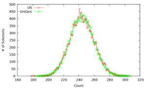
Figure 1: Uniformity comparison for case110

Table 1: Runtime performance comparison of 𝖴𝗇𝗂𝖦𝖾𝗇𝖴𝗇𝗂𝖦𝖾𝗇\mathsf{UniGen} and 𝖴𝗇𝗂𝖶𝗂𝗍𝖴𝗇𝗂𝖶𝗂𝗍\mathsf{UniWit}

A “*” entry indicates insufficient data for estimating success probability

Theorem 1 guarantees that the probability of generation of every witness lies within a specified tolerance of the uniform probability. In practice, however, the distribution of witnesses generated by 𝖴𝗇𝗂𝖦𝖾𝗇𝖴𝗇𝗂𝖦𝖾𝗇\mathsf{UniGen} is much more closer to a uniform distribution. To illustrate this, we implemented a uniform sampler, henceforth called 𝖴𝖲𝖴𝖲\mathsf{US}, and compared the distributions of witnesses generated by 𝖴𝗇𝗂𝖦𝖾𝗇𝖴𝗇𝗂𝖦𝖾𝗇\mathsf{UniGen} and by 𝖴𝖲𝖴𝖲\mathsf{US} for some representative benchmarks. Given a CNF formula F𝐹F, 𝖴𝖲𝖴𝖲\mathsf{US} first determines |RF|subscript𝑅𝐹|R_{F}| using an exact model counter (such as 𝗌𝗁𝖺𝗋𝗉𝖲𝖠𝖳𝗌𝗁𝖺𝗋𝗉𝖲𝖠𝖳\mathsf{sharpSAT}). To mimic generating a random witness, 𝖴𝖲𝖴𝖲\mathsf{US} simply generates a random number i𝑖i in {1​…​|RF|}1…subscript𝑅𝐹{1\ldots|R_{F}|}. To ensure fair comparison, we used the same source of randomness in both 𝖴𝗇𝗂𝖦𝖾𝗇𝖴𝗇𝗂𝖦𝖾𝗇\mathsf{UniGen} and 𝖴𝖲𝖴𝖲\mathsf{US}. For every problem instance on which the comparison was done, we generated a large number N𝑁N (=4×106absent4superscript106=4\times 10^{6}) of sample witnesses using each of 𝖴𝖲𝖴𝖲\mathsf{US} and 𝖴𝗇𝗂𝖦𝖾𝗇𝖴𝗇𝗂𝖦𝖾𝗇\mathsf{UniGen}. In each case, the number of times various witnesses were generated was recorded, yielding a distribution of the counts. Figure 1 shows the distributions of counts generated by 𝖴𝗇𝗂𝖦𝖾𝗇𝖴𝗇𝗂𝖦𝖾𝗇\mathsf{UniGen} and by 𝖴𝖲𝖴𝖲\mathsf{US} for one of our benchmarks (case110) with 16,384

1638416,384 witnesses. The horizontal axis represents counts and the vertical axis represents the number of witnesses appearing a specified number of times. Thus, the point (242,450)242450(242,450) represents the fact that each of 450450450 distinct witnesses were generated 242242242 times in 4×1064superscript1064\times 10^{6} runs. Observe that the distributions resulting from 𝖴𝗇𝗂𝖦𝖾𝗇𝖴𝗇𝗂𝖦𝖾𝗇\mathsf{UniGen} and 𝖴𝖲𝖴𝖲\mathsf{US} can hardly be distinguished in practice. This holds not only for this benchmark, but for all other benchmarks we experimented with.

Overall, our experiments confirm that 𝖴𝗇𝗂𝖦𝖾𝗇𝖴𝗇𝗂𝖦𝖾𝗇\mathsf{UniGen} is two to three orders of magnitude more efficient than state-of-the-art random witness generators, has probability of success almost 111, and preserves strong guarantees about the uniformity of generated witnesses. Furthermore, the distribution of generated witnesses can hardly be distinguished from that of a uniform sampler in practice.

Referring to the pseudocode of 𝖴𝗇𝗂𝖦𝖾𝗇𝖴𝗇𝗂𝖦𝖾𝗇\mathsf{UniGen} in Section 4, we observe that the only steps that depend directly on S𝑆S are those in line 141414, where hℎh is chosen randomly from Hx​o​r​(|S|,i,3)subscript𝐻𝑥𝑜𝑟𝑆𝑖3H_{xor}(|S|,i,3), and line 161616, where the set Y𝑌Y is computed by calling 𝖡𝖲𝖠𝖳𝖡𝖲𝖠𝖳\mathsf{BSAT}(F∧(h​(x1,…​x|S|)=α),hiThresh

𝐹ℎsubscript𝑥1…subscript𝑥𝑆𝛼hiThreshF\wedge(h(x_{1},\ldots x_{|S|})=\alpha),\mathrm{hiThresh}). Since all subsequent steps of the algorithm depend only on Y𝑌Y, it suffices to show that if S𝑆S is an independent support of F𝐹F, the probability distribution of Y𝑌Y obtained at line 161616 is identical to what we would obtain if S𝑆S was set equal to the entire support, X𝑋X, of F𝐹F.

Proof.

Since h′superscriptℎ′h^{\prime} is chosen uniformly at random from Hx​o​r​(n,i,3)subscript𝐻𝑥𝑜𝑟𝑛𝑖3H_{xor}(n,i,3), recalling the definition of Hx​o​r​(n,i,3)subscript𝐻𝑥𝑜𝑟𝑛𝑖3H_{xor}(n,i,3), we have F​(X→)∧(h′​(X→)=α′)𝐹→𝑋superscriptℎ′→𝑋superscript𝛼′F(\vec{X})\wedge(h^{\prime}(\vec{X})=\alpha^{\prime}) ≡\equiv F(X→)∧⋀l=1i((al,0⊕⨁j=1nal,j⋅x[j])↔α′[l])F(\vec{X})\wedge\bigwedge_{l=1}^{i}\left((a_{l,0}\oplus\bigoplus_{j=1}^{n}a_{l,j}\cdot x[j])\leftrightarrow\alpha^{\prime}[l]\right), where the al,jsubscript𝑎

𝑙𝑗a_{l,j}s are chosen independently and identically randomly from {0,1}01{0,1}.

Since S𝑆S is an independent support of F𝐹F, from Lemma 1, there exist Boolean functions g1,…​gn−k

subscript𝑔1…subscript𝑔𝑛𝑘g_{1},\ldots g_{n-k}, each with support S𝑆S, such that F(X→)→⋀j=1n−k(xk+j↔gj(S→))F(\vec{X})\rightarrow\bigwedge_{j=1}^{n-k}(x_{k+j}\leftrightarrow g_{j}(\vec{S})). Therefore, F​(X→)∧(h′​(X→)=α′)𝐹→𝑋superscriptℎ′→𝑋superscript𝛼′F(\vec{X})\wedge(h^{\prime}(\vec{X})=\alpha^{\prime}) is semantically equivalent to F(X→)∧⋀l=1i((al,0⊕⨁j=1kal,j⋅x[j]⊕B)↔α′[l])F(\vec{X})\wedge\bigwedge_{l=1}^{i}\left((a_{l,0}\oplus\bigoplus_{j=1}^{k}a_{l,j}\cdot x[j]\oplus B)\leftrightarrow\alpha^{\prime}[l]\right), where B≡⨁j=k+1nal,j⋅gj−k​(S→)𝐵superscriptsubscriptdirect-sum𝑗𝑘1𝑛⋅subscript𝑎

𝑙𝑗subscript𝑔𝑗𝑘→𝑆B\equiv\bigoplus_{j=k+1}^{n}a_{l,j}\cdot g_{j-k}(\vec{S}). Rearranging terms, we get F(X→)∧⋀l=1i((al,0⊕⨁j=1kal,j⋅x[j])↔(α′[l]⊕B))F(\vec{X})\wedge\bigwedge_{l=1}^{i}\left((a_{l,0}\oplus\bigoplus_{j=1}^{k}a_{l,j}\cdot x[j])\leftrightarrow(\alpha^{\prime}[l]\oplus B)\right).

Since α′superscript𝛼′\alpha^{\prime} is chosen uniformly at random from {0,1}isuperscript01𝑖{0,1}^{i} and since B𝐵B is independent of α′superscript𝛼′\alpha^{\prime}, it is easy to see that α′​[l]⊕Bdirect-sumsuperscript𝛼′delimited-[]𝑙𝐵\alpha^{\prime}[l]\oplus B is a random binary variable with equal probability of being 00 and 111. It follows that 𝖯𝗋​[𝖡𝖲𝖠𝖳​(F​(X→)∧(h′​(X→)=α′),t)=Y]𝖯𝗋delimited-[]𝖡𝖲𝖠𝖳𝐹→𝑋superscriptℎ′→𝑋superscript𝛼′𝑡𝑌\mathsf{Pr}\left[{\mathsf{BSAT}}(F(\vec{X})\wedge(h^{\prime}(\vec{X})=\alpha^{\prime}),t)=Y\right] == 𝖯𝗋​[𝖡𝖲𝖠𝖳​(F​(X→)∧(h​(S→)=α),t)=Y]𝖯𝗋delimited-[]𝖡𝖲𝖠𝖳𝐹→𝑋ℎ→𝑆𝛼𝑡𝑌\mathsf{Pr}\left[{\mathsf{BSAT}}(F(\vec{X})\wedge(h(\vec{S})=\alpha),t)=Y\right]. ∎

The next lemma provides a lower bound on the probability of generation of a witness. Let wi,y,αsubscript𝑤

𝑖𝑦𝛼w_{i,y,\alpha} denote the probability 𝖯𝗋[pivot1+κ\mathsf{Pr}\left[\frac{\mathrm{pivot}}{1+\kappa}\right. ≤|RF,h,α|≤1+(1+κ)​pivot​ and ​h​(y)=αabsentsubscript𝑅

𝐹ℎ𝛼11𝜅pivot and ℎ𝑦𝛼\left.\leq|R_{F,h,\alpha}|\leq 1+(1+\kappa)\mathrm{pivot}\mbox{ and }h(y)=\alpha\right. ::: h←𝑅Hx​o​r(n,i,3)]\left.h\xleftarrow{R}H_{xor}(n,i,3)\right]. The proof of the lemma also provides a lower bound on wm,y,αsubscript𝑤

𝑚𝑦𝛼w_{m,y,\alpha}.

Proof.

If |RF|≤1+(1+κ)​pivotsubscript𝑅𝐹11𝜅pivot|R_{F}|\leq 1+(1+\kappa)\mathrm{pivot}, the lemma holds trivially (see lines 555–777 of the pseudocode). Suppose |RF|≥1+(1+κ)​pivotsubscript𝑅𝐹11𝜅pivot|R_{F}|\geq 1+(1+\kappa)\mathrm{pivot} and let U𝑈U denote the event that witness y∈RF𝑦subscript𝑅𝐹y\in R_{F} is output by 𝖴𝗇𝗂𝖦𝖾𝗇𝖴𝗇𝗂𝖦𝖾𝗇\mathsf{UniGen} on inputs F𝐹F, ε𝜀\varepsilon and X𝑋X. Let pi,ysubscript𝑝

𝑖𝑦p_{i,y} denote the probability that we return from line 171717 for a particular value of i𝑖i with y𝑦y in RF,h,αsubscript𝑅

𝐹ℎ𝛼R_{F,h,\alpha}, where α∈{0,1}i𝛼superscript01𝑖\alpha\in{0,1}^{i} is the value chosen in line 151515. Then, 𝖯𝗋​[U]=∑i=q−3q1|Y|​pi,y​∏j=q−3i−1(1−pj,y)𝖯𝗋delimited-[]𝑈superscriptsubscript𝑖𝑞3𝑞1𝑌subscript𝑝

𝑖𝑦superscriptsubscriptproduct𝑗𝑞3𝑖11subscript𝑝

𝑗𝑦\mathsf{Pr}[U]=\sum_{i=q-3}^{q}\frac{1}{|Y|}p_{i,y}\prod_{j=q-3}^{i-1}(1-p_{j,y}), where Y𝑌Y is the set of witnesses returned by 𝖡𝖲𝖠𝖳𝖡𝖲𝖠𝖳\mathsf{BSAT} in line 161616 of the pseudocode. Let fm=𝖯𝗋​[q−3≤m≤q]subscript𝑓𝑚𝖯𝗋delimited-[]𝑞3𝑚𝑞f_{m}=\mathsf{Pr}[q-3\leq m\leq q]. From Lemma 3, we know that fm≥0.8subscript𝑓𝑚0.8f_{m}\geq 0.8. From the design of the algorithm, we also know that 11+κ​pivot≤|Y|≤1+(1+κ)​pivot11𝜅pivot𝑌11𝜅pivot\frac{1}{1+\kappa}\mathrm{pivot}\leq|Y|\leq 1+(1+\kappa)\mathrm{pivot}. Therefore, 𝖯𝗋​[U]≥11+(1+κ)​pivot⋅pm,y⋅fm𝖯𝗋delimited-[]𝑈⋅111𝜅pivotsubscript𝑝

𝑚𝑦subscript𝑓𝑚\mathsf{Pr}[U]\geq\frac{1}{1+(1+\kappa)\mathrm{pivot}}\cdot p_{m,y}\cdot f_{m}. The proof is now completed by showing pm,y≥12m​(1−e−1)subscript𝑝

𝑚𝑦1superscript2𝑚1superscript𝑒1p_{m,y}\geq\frac{1}{2^{m}}(1-e^{-1}). This gives 𝖯𝗋​[U]≥0.8​(1−e−1)(1+(1+κ)​p​i​v​o​t)​2m≥0.8​(1−e−1)(1.06+κ)​(|RF|−1)𝖯𝗋delimited-[]𝑈0.81superscript𝑒111𝜅𝑝𝑖𝑣𝑜𝑡superscript2𝑚0.81superscript𝑒11.06𝜅subscript𝑅𝐹1\mathsf{Pr}[U]\geq\frac{0.8(1-e^{-1})}{(1+(1+\kappa)pivot)2^{m}}\geq\frac{0.8(1-e^{-1})}{(1.06+\kappa)(|R_{F}|-1)}. The last inequality uses the observation that 1/pivot≤0.061pivot0.061/\mathrm{pivot}\leq 0.06.

To calculate pm,ysubscript𝑝

𝑚𝑦p_{m,y}, we first note that since y∈RF𝑦subscript𝑅𝐹y\in R_{F}, the requirement “y∈RF,h,α𝑦subscript𝑅

𝐹ℎ𝛼y\in R_{F,h,\alpha}" reduces to “y∈h−1​(α)𝑦superscriptℎ1𝛼y\in h^{-1}(\alpha)". For α∈{0,1}n𝛼superscript01𝑛\alpha\in{0,1}^{n}, we define wm,y,αsubscript𝑤

𝑚𝑦𝛼w_{m,y,\alpha} as 𝖯𝗋[pivot1+κ\mathsf{Pr}\left[\frac{\mathrm{pivot}}{1+\kappa}\right. ≤|RF,h,α|≤1+(1+κ)absentsubscript𝑅

𝐹ℎ𝛼11𝜅\left.\leq|R_{F,h,\alpha}|\leq 1+(1+\kappa)\right. pivot and h(y)=α:h←𝑅Hx​o​r(n,m,3)]\left.pivot\mbox{ and }h(y)=\alpha:h\xleftarrow{R}H_{xor}(n,m,3)\right]. Therefore, pm,ysubscript𝑝

𝑚𝑦p_{m,y} =Σα∈{0,1}m​(wm,y,α​.2−m)absentsubscriptΣ𝛼superscript01𝑚subscript𝑤

𝑚𝑦𝛼superscript.2𝑚=\Sigma_{\alpha\in{0,1}^{m}}\left(w_{m,y,\alpha}.2^{-m}\right). The proof is now completed by showing that wm,y,α≥(1−e−1)/2msubscript𝑤

𝑚𝑦𝛼1superscript𝑒1superscript2𝑚w_{m,y,\alpha}\geq(1-e^{-1})/2^{m} for every α∈{0,1}m𝛼superscript01𝑚\alpha\in{0,1}^{m} and y∈{0,1}n𝑦superscript01𝑛y\in{0,1}^{n}.

Towards this end, let us first fix a random y𝑦y. Now we define an indicator variable γz,αsubscript𝛾

𝑧𝛼\gamma_{z,\alpha} for every z∈RF∖{y}𝑧subscript𝑅𝐹𝑦z\in R_{F}\setminus{y} such that γz,α=1subscript𝛾

𝑧𝛼1\gamma_{z,\alpha}=1 if h​(z)=αℎ𝑧𝛼h(z)=\alpha, and γz,α=0subscript𝛾

𝑧𝛼0\gamma_{z,\alpha}=0 otherwise. Let us fix α𝛼\alpha and choose hℎh uniformly at random from Hx​o​r​(n,m,3)subscript𝐻𝑥𝑜𝑟𝑛𝑚3H_{xor}(n,m,3). The random choice of h induces a probability distribution on γz,αsubscript𝛾

𝑧𝛼\gamma_{z,\alpha} such that E​[γz,α]=𝖯𝗋​[γz,α=1]=2−m𝐸delimited-[]subscript𝛾

𝑧𝛼𝖯𝗋delimited-[]subscript𝛾

𝑧𝛼1superscript2𝑚E[\gamma_{z,\alpha}]=\mathsf{Pr}[\gamma_{z,\alpha}=1]=2^{-m}. Since we have fixed y𝑦y, and since hash functions chosen from Hx​o​r​(n,m,3)subscript𝐻𝑥𝑜𝑟𝑛𝑚3H_{xor}(n,m,3) are 333-wise independent, it follows that for every distinct za,zb∈RF∖{y}

subscript𝑧𝑎subscript𝑧𝑏 subscript𝑅𝐹𝑦z_{a},z_{b}\in R_{F}\setminus{y}, the random variables γza,α,γzb,α

subscript𝛾

subscript𝑧𝑎𝛼subscript𝛾

subscript𝑧𝑏𝛼\gamma_{z_{a},\alpha},\gamma_{z_{b},\alpha} are 2-wise independent. Let Γα=∑z∈RF∖{y}γz,αsubscriptΓ𝛼subscript𝑧subscript𝑅𝐹𝑦subscript𝛾

𝑧𝛼\Gamma_{\alpha}=\sum_{z\in R_{F}\setminus{y}}\gamma_{z,\alpha} and μα=E​[Γα]subscript𝜇𝛼𝐸delimited-[]subscriptΓ𝛼\mu_{\alpha}=E[\Gamma_{\alpha}]. Clearly, Γα=|RF,h,α|−1subscriptΓ𝛼subscript𝑅

𝐹ℎ𝛼1\Gamma_{\alpha}=|R_{F,h,\alpha}|-1 and μα=∑z∈RF∖{y}subscript𝜇𝛼subscript𝑧subscript𝑅𝐹𝑦\mu_{\alpha}=\sum_{z\in R_{F}\setminus{y}} E​[γz,α]𝐸delimited-[]subscript𝛾

𝑧𝛼E[\gamma_{z,\alpha}] =|RF|−12mabsentsubscript𝑅𝐹1superscript2𝑚=\frac{|R_{F}|-1}{2^{m}}. Also, 𝖯𝗋​[pivot1+κ≤|RF,h,α|≤1+(1+κ)​pivot]𝖯𝗋delimited-[]pivot1𝜅subscript𝑅

𝐹ℎ𝛼11𝜅pivot\mathsf{Pr}[\frac{\mathrm{pivot}}{1+\kappa}\leq|R_{F,h,\alpha}|\leq 1+(1+\kappa)\mathrm{pivot}] =𝖯𝗋​[pivot1+κ−1≤|RF,h,α|−1≤(1+κ)​pivot]absent𝖯𝗋delimited-[]pivot1𝜅1subscript𝑅

𝐹ℎ𝛼11𝜅pivot=\mathsf{Pr}[\frac{\mathrm{pivot}}{1+\kappa}-1\leq|R_{F,h,\alpha}|-1\leq(1+\kappa)\mathrm{pivot}] ≥𝖯𝗋​[pivot1+κ≤|RF,h,α|−1≤(1+κ)​pivot]absent𝖯𝗋delimited-[]pivot1𝜅subscript𝑅

𝐹ℎ𝛼11𝜅pivot\geq\mathsf{Pr}[\frac{\mathrm{pivot}}{1+\kappa}\leq|R_{F,h,\alpha}|-1\leq(1+\kappa)\mathrm{pivot}]. Using the expression for pivotpivot\mathrm{pivot}, we get 2≤⌊e−1/2​(1+1/ϵ)2⋅|RF|−12m⌋2⋅superscript𝑒12superscript11italic-ϵ2subscript𝑅𝐹1superscript2𝑚2\leq\lfloor e^{-1/2}(1+1/\epsilon)^{2}\cdot\frac{|R_{F}|-1}{2^{m}}\rfloor. Therefore using Theorem 1 and substituting pivot=(|RF|−1)/2mpivotsubscript𝑅𝐹1superscript2𝑚\mathrm{pivot}=(|R_{F}|-1)/2^{m}, we get 𝖯𝗋​[pivot1+κ≤|RF,h,α|−1≤(1+κ)​pivot]≥1−e−1𝖯𝗋delimited-[]pivot1𝜅subscript𝑅

𝐹ℎ𝛼11𝜅pivot1superscript𝑒1\mathsf{Pr}[\frac{\mathrm{pivot}}{1+\kappa}\leq|R_{F,h,\alpha}|-1\leq(1+\kappa)\mathrm{pivot}]\geq 1-e^{-1}. Therefore, 𝖯𝗋​[pivot1+κ≤|RF,h,α|≤1+(1+κ)​pivot]≥1−e−1𝖯𝗋delimited-[]pivot1𝜅subscript𝑅

𝐹ℎ𝛼11𝜅pivot1superscript𝑒1\mathsf{Pr}[\frac{\mathrm{pivot}}{1+\kappa}\leq|R_{F,h,\alpha}|\leq 1+(1+\kappa)\mathrm{pivot}]\geq 1-e^{-1} Since hℎh is chosen at random from Hx​o​r​(n,m,3)subscript𝐻𝑥𝑜𝑟𝑛𝑚3H_{xor}(n,m,3), we also have 𝖯𝗋​[h​(y)=α]=1/2m𝖯𝗋delimited-[]ℎ𝑦𝛼1superscript2𝑚\mathsf{Pr}[h(y)=\alpha]=1/2^{m}. It follows that wm,y,α≥(1−e−1)/2msubscript𝑤

𝑚𝑦𝛼1superscript𝑒1superscript2𝑚w_{m,y,\alpha}\geq(1-e^{-1})/2^{m}. ∎

Proof.

We will use the terminology introduced in the proof of Lemma 4. Clearly, μα=|RF|−12isubscript𝜇𝛼subscript𝑅𝐹1superscript2𝑖\mu_{\alpha}=\frac{|R_{F}|-1}{2^{i}}. Since each γz,αsubscript𝛾

𝑧𝛼\gamma_{z,\alpha} is a 00-111 variable, 𝖵​[γz,α]≤𝖤​[γz,α]𝖵delimited-[]subscript𝛾

𝑧𝛼𝖤delimited-[]subscript𝛾

𝑧𝛼\mathsf{V}\left[\gamma_{z,\alpha}\right]\leq\mathsf{E}\left[\gamma_{z,\alpha}\right]. Therefore, σz,α2subscriptsuperscript𝜎2

𝑧𝛼\sigma^{2}_{z,\alpha} ≤∑z≠y,z∈RF𝖤​[γz,α]absentsubscriptformulae-sequence𝑧𝑦𝑧subscript𝑅𝐹𝖤delimited-[]subscript𝛾

𝑧𝛼\leq\sum_{z\neq y,z\in R_{F}}\mathsf{E}\left[\gamma_{z,\alpha}\right] ≤∑z∈RF𝖤​[γz,α]absentsubscript𝑧subscript𝑅𝐹𝖤delimited-[]subscript𝛾

𝑧𝛼\leq\sum_{z\in R_{F}}\mathsf{E}\left[\gamma_{z,\alpha}\right] =𝖤​[Γα]=2−m​(|RF|−1)absent𝖤delimited-[]subscriptΓ𝛼superscript2𝑚subscript𝑅𝐹1=\mathsf{E}\left[\Gamma_{\alpha}\right]=2^{-m}(|R_{F}|-1). So 𝖯𝗋​[p​i​v​o​t1+κ≤|RF,h,α|≤1+(1+κ)​pivot]≤𝖯𝗋​[|RF,h,α|−1≤(1+κ)​pivot]𝖯𝗋delimited-[]𝑝𝑖𝑣𝑜𝑡1𝜅subscript𝑅

𝐹ℎ𝛼11𝜅pivot𝖯𝗋delimited-[]subscript𝑅

𝐹ℎ𝛼11𝜅pivot\mathsf{Pr}[\frac{pivot}{1+\kappa}\leq|R_{F,h,\alpha}|\leq 1+(1+\kappa)\mathrm{pivot}]\leq\mathsf{Pr}[|R_{F,h,\alpha}|-1\leq(1+\kappa)\mathrm{pivot}]. From Chebyshev’s inequality, we know that 𝖯𝗋[|Γα−μz,α|≥\mathsf{Pr}\left[|\Gamma_{\alpha}-\mu_{z,\alpha}|\geq\right. κσz,α]≤1/κ2\left.\kappa\sigma_{z,\alpha}\right]\leq 1/\kappa^{2} for every κ>0𝜅0\kappa>0. By choosing κ=(1−1+κ2m−i)​μz,ασz,α𝜅11𝜅superscript2𝑚𝑖subscript𝜇

𝑧𝛼subscript𝜎

𝑧𝛼\kappa=(1-\frac{1+\kappa}{2^{m-i}})\frac{\mu_{z,\alpha}}{\sigma_{z,\alpha}}, we have 𝖯𝗋​[|RF,h,α|−1≤(1+κ)​pivot]𝖯𝗋delimited-[]subscript𝑅

𝐹ℎ𝛼11𝜅pivot\mathsf{Pr}[|R_{F,h,\alpha}|-1\leq(1+\kappa)\mathrm{pivot}] ≤𝖯𝗋absent𝖯𝗋\leq\mathsf{Pr} [|(|RF,h,α|−1)−|RF|−12i|\left[|(|R_{F,h,\alpha}|-1)-\frac{|R_{F}|-1}{2^{i}}|\right. ≥(1−1+κ2m−i)|RF|−12i]\left.\geq(1-\frac{1+\kappa}{2^{m-i}})\frac{|R_{F}|-1}{2^{i}}\right] ≤1(1−(1+κ)2m−i)2⋅2i|RF|−1absent⋅1superscript11𝜅superscript2𝑚𝑖2superscript2𝑖subscript𝑅𝐹1\leq\frac{1}{\left(1-\frac{(1+\kappa)}{2^{m-i}}\right)^{2}}\cdot\frac{2^{i}}{|R_{F}|-1}. Since hℎh is chosen at random from Hx​o​r​(n,m,3)subscript𝐻𝑥𝑜𝑟𝑛𝑚3H_{xor}(n,m,3), we also have 𝖯𝗋​[h​(y)=α]=1/2i𝖯𝗋delimited-[]ℎ𝑦𝛼1superscript2𝑖\mathsf{Pr}[h(y)=\alpha]=1/2^{i}. It follows that wi,y,α≤1|RF|−1​1(1−1+κ2m−i)2subscript𝑤

𝑖𝑦𝛼1subscript𝑅𝐹11superscript11𝜅superscript2𝑚𝑖2w_{i,y,\alpha}\leq\frac{1}{|R_{F}|-1}\frac{1}{\left(1-\frac{1+\kappa}{2^{m-i}}\right)^{2}}. The bound for pi,ysubscript𝑝

𝑖𝑦p_{i,y} is easily obtained by noting that pi,y=Σα∈{0,1}i​(wi,y,α​.2−i)subscript𝑝

𝑖𝑦subscriptΣ𝛼superscript01𝑖subscript𝑤

𝑖𝑦𝛼superscript.2𝑖p_{i,y}=\Sigma_{\alpha\in{0,1}^{i}}\left(w_{i,y,\alpha}.2^{-i}\right). ∎

Proof.

If |RF|≤1+(1+κ)​pivotsubscript𝑅𝐹11𝜅pivot|R_{F}|\leq 1+(1+\kappa)\mathrm{pivot}, the theorem holds trivially. Suppose |RF|>1+(1+κ)​pivotsubscript𝑅𝐹11𝜅pivot|R_{F}|>1+(1+\kappa)\mathrm{pivot} and let Psuccsubscript𝑃succP_{\mathrm{succ}} denote the probability that a run of the algorithm 𝖴𝗇𝗂𝖦𝖾𝗇𝖴𝗇𝗂𝖦𝖾𝗇\mathsf{UniGen} succeeds. Let pi,subscript𝑝𝑖p_{i}, such that (q−3≤i≤q)𝑞3𝑖𝑞(q-3\leq i\leq q) denote the conditional probability that 𝖴𝗇𝗂𝖦𝖾𝗇𝖴𝗇𝗂𝖦𝖾𝗇\mathsf{UniGen} (F𝐹F, ε𝜀\varepsilon, X𝑋X) terminates in iteration i𝑖i of the repeat-until loop (line 11-16) with pivot1+κ≤|RF,h,α|≤1+(1+κ)​pivotpivot1𝜅subscript𝑅

𝐹ℎ𝛼11𝜅pivot\frac{\mathrm{pivot}}{1+\kappa}\leq|R_{F,h,\alpha}|\leq 1+(1+\kappa)\mathrm{pivot}, given |RF|>1+(1+κ)​pivotsubscript𝑅𝐹11𝜅pivot|R_{F}|>1+(1+\kappa)\mathrm{pivot}. Therefore, Psucc=∑i=q−3qpi​∏j=q−3i(1−pj)subscript𝑃succsuperscriptsubscript𝑖𝑞3𝑞subscript𝑝𝑖superscriptsubscriptproduct𝑗𝑞3𝑖1subscript𝑝𝑗P_{\mathrm{succ}}=\sum_{i=q-3}^{q}p_{i}\prod_{j=q-3}^{i}(1-p_{j}). Let fm=𝖯𝗋​[q−3≤m≤q]subscript𝑓𝑚𝖯𝗋delimited-[]𝑞3𝑚𝑞f_{m}=\mathsf{Pr}[q-3\leq m\leq q]. Therefore, Psucc≥pm​fm≥0.8​pmsubscript𝑃succsubscript𝑝𝑚subscript𝑓𝑚0.8subscript𝑝𝑚P_{\mathrm{succ}}\geq p_{m}f_{m}\geq 0.8p_{m}. The theorem is now proved by using Theorem 1 to show that pm≥1−e−3/2≥0.77subscript𝑝𝑚1superscript𝑒320.77p_{m}\geq 1-e^{-3/2}\geq 0.77.

For every y∈{0,1}n𝑦superscript01𝑛y\in{0,1}^{n} and for every α∈{0,1}m𝛼superscript01𝑚\alpha\in{0,1}^{m}, define an indicator variable νy,αsubscript𝜈

𝑦𝛼\nu_{y,\alpha} as follows: νy,α=1subscript𝜈

𝑦𝛼1\nu_{y,\alpha}=1 if h​(y)=αℎ𝑦𝛼h(y)=\alpha, and νy,α=0subscript𝜈

𝑦𝛼0\nu_{y,\alpha}=0 otherwise. Let us fix α𝛼\alpha and y𝑦y and choose hℎh uniformly at random from Hx​o​r​(n,m,3)subscript𝐻𝑥𝑜𝑟𝑛𝑚3H_{xor}(n,m,3). The random choice of hℎh induces a probability distribution on νy,αsubscript𝜈

𝑦𝛼\nu_{y,\alpha}, such that 𝖯𝗋​[νy,α=1]=𝖯𝗋​[h​(y)=α]=2−m𝖯𝗋delimited-[]subscript𝜈

𝑦𝛼1𝖯𝗋delimited-[]ℎ𝑦𝛼superscript2𝑚\mathsf{Pr}[\nu_{y,\alpha}=1]=\mathsf{Pr}[h(y)=\alpha]=2^{-m} and 𝖤​[νy,α]=𝖯𝗋​[νy,α=1]=2−m𝖤delimited-[]subscript𝜈

𝑦𝛼𝖯𝗋delimited-[]subscript𝜈

𝑦𝛼1superscript2𝑚\mathsf{E}[\nu_{y,\alpha}]=\mathsf{Pr}[\nu_{y,\alpha}=1]=2^{-m}. In addition 3-wise independence of hash functions chosen from Hx​o​r​(n,m,3)subscript𝐻𝑥𝑜𝑟𝑛𝑚3H_{xor}(n,m,3) implies that for every distinct ya,yb,yc∈RF

subscript𝑦𝑎subscript𝑦𝑏subscript𝑦𝑐 subscript𝑅𝐹y_{a},y_{b},y_{c}\in R_{F}, the random variables νya,α,νyb,α

subscript𝜈

subscript𝑦𝑎𝛼subscript𝜈

subscript𝑦𝑏𝛼\nu_{y_{a},\alpha},\nu_{y_{b},\alpha} and νyc,αsubscript𝜈

subscript𝑦𝑐𝛼\nu_{y_{c},\alpha} are 3-wise independent.

Let Γα=∑y∈RFνy,αsubscriptΓ𝛼subscript𝑦subscript𝑅𝐹subscript𝜈

𝑦𝛼\Gamma_{\alpha}=\sum_{y\in R_{F}}\nu_{y,\alpha} and μα=𝖤​[Γα]subscript𝜇𝛼𝖤delimited-[]subscriptΓ𝛼\mu_{\alpha}=\mathsf{E}\left[\Gamma_{\alpha}\right]. Clearly, Γα=|RF,h,α|subscriptΓ𝛼subscript𝑅

𝐹ℎ𝛼\Gamma_{\alpha}=|R_{F,h,\alpha}| and μα=∑y∈RF𝖤​[νy,α]=2−m​|RF|subscript𝜇𝛼subscript𝑦subscript𝑅𝐹𝖤delimited-[]subscript𝜈

𝑦𝛼superscript2𝑚subscript𝑅𝐹\mu_{\alpha}=\sum_{y\in R_{F}}\mathsf{E}\left[\nu_{y,\alpha}\right]=2^{-m}|R_{F}|. Since |RF|>𝑝𝑖𝑣𝑜𝑡subscript𝑅𝐹𝑝𝑖𝑣𝑜𝑡|R_{F}|>\mathit{pivot} and i−l>0𝑖𝑙0i-l>0, using the expression for 𝑝𝑖𝑣𝑜𝑡𝑝𝑖𝑣𝑜𝑡\mathit{pivot}, we get 3≤⌊e−1/2​(1+1ε)−2⋅|RF|2m⌋3⋅superscript𝑒12superscript11𝜀2subscript𝑅𝐹superscript2𝑚3\leq\left\lfloor e^{-1/2}(1+\frac{1}{\varepsilon})^{-2}\cdot\frac{|R_{F}|}{2^{m}}\right\rfloor. Therefore, using Theorem 1, 𝖯𝗋[|RF|2m.(1−κ1+κ)≤|RF,h,α|\mathsf{Pr}\left[\frac{|R_{F}|}{2^{m}}.\left(1-\frac{\kappa}{1+\kappa}\right)\leq|R_{F,h,\alpha}|\right. ≤(1+κ)|RF|2m]>1−e−3/2\left.\leq(1+\kappa)\frac{|R_{F}|}{2^{m}}\right]>1-e^{-3/2}. Simplifying and noting that κ1+κ<κ𝜅1𝜅𝜅\frac{\kappa}{1+\kappa}<\kappa for all κ>0𝜅0\kappa>0, we obtain 𝖯𝗋[(1+κ)−1⋅|RF|2m≤|RF,h,α|\mathsf{Pr}\left[(1+\kappa)^{-1}\cdot\frac{|R_{F}|}{2^{m}}\leq|R_{F,h,\alpha}|\right. ≤(1+κ)⋅|RF|2m]>1−e−3/2\left.\leq(1+\kappa)\cdot\frac{|R_{F}|}{2^{m}}\right]>1-e^{-3/2}. Also, pivot1+κ=11+κ​|RF|−12m≤|RF|(1+κ)​2mpivot1𝜅11𝜅subscript𝑅𝐹1superscript2𝑚subscript𝑅𝐹1𝜅superscript2𝑚\frac{\mathrm{pivot}}{1+\kappa}=\frac{1}{1+\kappa}\frac{|R_{F}|-1}{2^{m}}\leq\frac{|R_{F}|}{(1+\kappa)2^{m}} and 1+(1+κ)​pivot=1+(1+κ)​(|RF|−1)2m≥(1+κ)​|RF|2m11𝜅pivot11𝜅subscript𝑅𝐹1superscript2𝑚1𝜅subscript𝑅𝐹superscript2𝑚1+(1+\kappa)\mathrm{pivot}=1+\frac{(1+\kappa)(|R_{F}|-1)}{2^{m}}\geq\frac{(1+\kappa)|R_{F}|}{2^{m}}. Therefore, pm=𝖯𝗋​[pivot1+κ≤|RF,h,α|≤1+(1+κ)​pivot]≥subscript𝑝𝑚𝖯𝗋delimited-[]pivot1𝜅subscript𝑅

𝐹ℎ𝛼11𝜅pivotabsentp_{m}=\mathsf{Pr}[\frac{\mathrm{pivot}}{1+\kappa}\leq|R_{F,h,\alpha}|\leq 1+(1+\kappa)\mathrm{pivot}]\geq 𝖯𝗋[(1+κ)−1⋅|RF|2m\mathsf{Pr}\left[(1+\kappa)^{-1}\cdot\frac{|R_{F}|}{2^{m}}\right. ≤|RF,h,α|absentsubscript𝑅

𝐹ℎ𝛼\left.\leq|R_{F,h,\alpha}|\right. ≤(1+κ)⋅|RF|2m]≥1−e−3/2\left.\leq(1+\kappa)\cdot\frac{|R_{F}|}{2^{m}}\right]\geq 1-e^{-3/2}. ∎